In customer feedback we often run the same survey to different sets of respondents and we are very interested in identifying whether the responses are different between different groups. Typically those groups are either different sub-segments (male vs female customers) or different time periods (last quarter vs this quarter).

However, too often the different/not-different determination is done overly simplistically using a simple average of the feedback scores. If the sample average is different then we assume the group average is different. If it’s the same we assume the group average is the same.

While simple is often good, in this case the risk of making a false positive or false negative error can be high. The cost of that error can be substantial: changes that are actually working can be discontinued (false negative) or initiatives that are not working continued (false positive).

So while it is tempting to just look at whether the average score has changed we need to do a little more work to validate that decision.

Enter Student’s t-Test (Independent)

Nothing to do with education, Student’s t-test was named for its inventor’s pen name and is a relatively straightforward test you can perform on data to determine if there is a difference between two sets of customer feedback responses.

Assumptions

As you might expect there are quite a few assumptions when using this test but they are assumptions that are usually valid when applied to customer feedback so you should be fine:

1. Normal Distribution: The data needs to be normally distributed. This is usually the case in customer feedback data.
2. Homogeneity of variance: The variance between the two samples needs to be the same. Again this is commonly the case for feedback data in the situations we will look at below.
3. Data is independent: For our purposes we will be using an independent t-test and that means that the samples should be independent of each other. For instance, you should not survey the same people in each sample. Again we are normally fine on this assumption for sample based time period surveys as the chance of exactly the same people responding to each survey is low.
4. Random samples: The process of taking the sample should be exactly random, i.e.the chance of receiving a response from every person should be exactly the same. Now we know in practice that there is some skewing of the response curve because very happy and very unhappy clients are more inclined to respond than those in the centre. For this assumption we probably just have to accept that the sample is not truly random.
5. Data must be continuous: In general the data we deal with in customer feedback is Ordinal data:

“How responsive is Company X in closing the loop after problem resolution? Where 1 is very unresponsive and 5 is very responsive”

The response is one of 5 numbers. Now technically you should not use the t-test for this type of data but there is quite a lot of statistical discussion that indicates it’s perfectly fine to do so.

What Can You Test?

The t-test test compares the two samples and provides the probability that they have the same mean.

Commonly you would test for changes in the overall score (“would recommend” question, customer satisfaction, customer effort score, etc.) and the scores for the different attributes in your customer feedback questions: responsiveness, accuracy, professionalism, etc. The questions are typically on a scale with a number as a response.

Note that this test does not work for Net Promoter Score: see this article for more information on how to test for changes in NPS.

As noted before, the test can be used for changes over time (monthly numbers) or between groups (contact centre team A and contact centre team B).

Using Excel

For the detailed maths you can check out Wikipedia but here I am going to simply show you how to do the calculation in Excel as this is what most people will use.

Step 1: Get Your Data and Run the Test

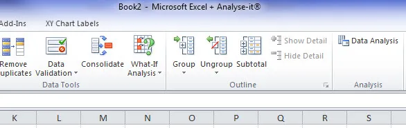
Below we have some sample data that shows the response scores for 3 months along with their average.

Looking at the simple average some people would be inclined to say that the score rose each month 3.4 -> 3.6 -> 4.7. Maybe, maybe not. Before we make any big decisions based on that information let’s test it and find out.

First we’ll compare May and June to see if there was change in the score.

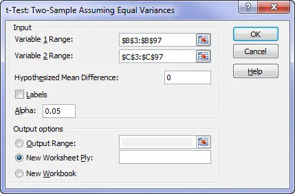
From the Data menu in Excel, select Data analysis and you will be presented with the selection box. Scroll down to “t-Test: Two Sample Assuming Equal Variances”.

Enter the data for the first and second range of responses. These are your two datasets and in our case are May and June but for you could be Team A and Team B, etc.

Set the hypothesised mean difference to 0 (zero) (we are testing for no difference) and put the output range to where ever you would like. Hit Okay and Excel does the work.

Step 2: Interpret the Result

This is the result of the May to June test. As you can see there are lot of data provided in the results. The trick is to find the information that you really care about and that’s right at the bottom: “P(T<=t) two-tail”

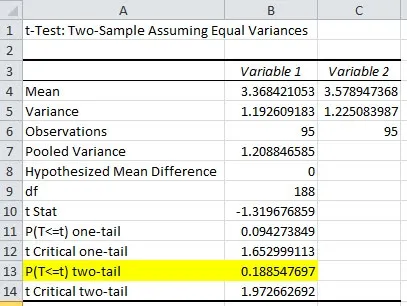
This value is the probability that the two populations have the same mean and that the difference in the sample means (3.4 to 3.6) is simply statistical noise. This probability is 18.8% for our example.

In statistics we generally use 5% probability as the decision point (don’t ask why). So based on this test, because the probability that they are the same is 18.8% (i.e. greater than 5%) we would accept that they are the same.

Aside: This is termed accepting the null hypothesis.

Now let’s look at the June and July data.

Here we can see that the probability that the two populations are the same is 0.00000000135%. As that is less than 5% (by a long way) we will decide that there really has been a change in the average for the underlying population.

Aside: This is termed rejecting the null hypothesis.

Handy Dandy Interpretation Summary for t-Test in Excel

The handy dandy summary card for this test:

• If “P(T<=t) two-tail” < 5% then a change has probably occurred in the overall population
• “If P(T<=t) two-tail” > 5% then a change has probably NOT occurred in the overall population

Conclusion

Too often when reviewing customer feedback data and looking at charts people see changes in the sample average score and then interpret that the overall response of all customers has changed. This causes them to make poor decisions and spend hours trying to find the “reason” that the change occurred.

Don’t make that mistake.

A 30 second t-Test can validate if change has probably occurred and allow you to confidently state: “yes it has increased”, or, “I know it looks like it’s increased up but it’s not a significant change and we should ignore it.”